Markov Chains

What is a Markov Chain?

---

A Markov Chain is a discrete-time stochastic process that can be in some state at any time. For any discrete time t and all states, a Markov Chain is the probability of moving to a future state given the current state, but does not depend on the states the chain passed through on the way to the current state, giving it a memoryless property.

To understand a memoryless property, we can do a weather modeling example. Let’s say a weather model has two states: Sunny and Rainy. If a system has memory, hence a non-Markovian system, we can say that the chance of rain tomorrow depends on whether it rained today and if it rained yesterday. Now, if a system has no memory, hence a Markovian system, we can say the chance of rain tomorrow depends only on whether it is raining today. So, it does not matter if it was Sunny for he past 10 days or if it was raining yesterday in a Markovian system. You can model this as:

\( P(X_{t+1} = i_{t+1} | X_t=i_t, X_{t-1}=i_{t-1}, \dots{},X_i=i_t, X_0=i_0) = P(X_{t+1} = j |X_t=i_t) \)

This says that knowing the entire past history gives you no additional information beyond knowing just the current state.

We assume that for all states i and j that this equation is independent of t, which gives us:

\(P(X_{t+1} = j |X_t=i_t) = p_{ij}\)

Which is the probability that given the system is in state i at time t, it will be in state j at the next time step.

Now, if the system moves from some one state to another, we can model that with a transition probability matrix, which is where all the transition probabilities live of the next state given current state:

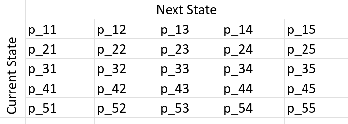
What if a Markov Chain is in a certain state at a certain time and we want to find the probability that the Markov Chain will be in another state n periods later?

Let’s say you want to find the probability of a state j two periods from now, starting in your current state i. All you need to do is take your probability matrix, put it to the n-th power (2nd power in this case), and take your result from row i and column j. This is the general formula for that:

\(P_{ij}(n) = ij\text{th element of }P^n\)

Key Terms to Classify Markov Chain

---

• Path: Sequence of transitions where each transition has a positive probability of occurring.

• Reachable: A state j is reachable from another state i if there is a path leading from i to j.

• Communicate: Two states communicate if state i is reachable from state j, and state j is reachable from state i.

• Absorbing: A state i is an absorbing state if the probability of the row i and column i value is 1.

• Transient: If there is a state j that is reachable from state i, but state i is not reachable from state j, then state i is a transient state.

• Recurrent: If a state is not transient, it is a recurrent state.

• Periodic: All paths leading from a state i back to state i have a length that is a multiple of period k (which is > 1 if it’s the smallest number). If a recurrent state is not periodic, then it’s aperiodic.

• Ergodic: If all states in a chain are recurrent, aperiodic, and communicate with each other, the chain is ergodic.

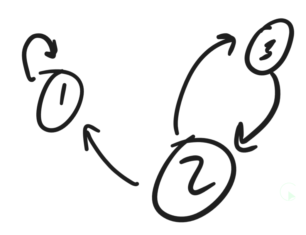
In the image above, state 2 is transient because it can go to state 1 but state 2 is not reachable from state 1. It also looks like state 1 becomes an absorbing state as soon as it enters state 1 from state 2.

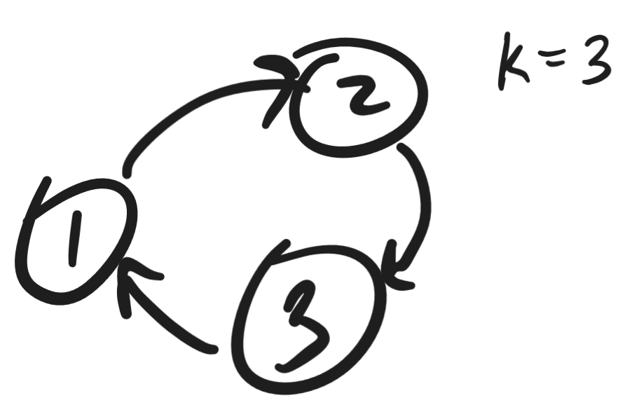
This image is a periodic Markov Chain. The length is 3 because if you start from state 1 (or any of the states), the path would be 1→2→3→1, so it would take 3 transitions to get back to state 1. So, if you start from state 1, it takes 3, 6, 9, etc., all multiples of 3 steps to get back to state 1. Let’s look at a more complex periodic chain.

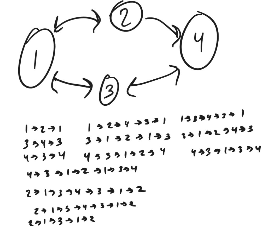
I wrote all the transitions down and you can see that the smallest length is 2, which is > 1. So, every other length should be a multiple of 2. If we look at the other two paths of when starting at state 1, they are lengths of 4, which is a multiple of 2. If we look at the last path when starting at state 4, the length is 6, which is a multiple of 2.

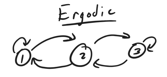
• All states communicate because every state is reachable because there is a path from each state to get back to that same state.

• If a state has a self-loop, the chain is automatically aperiodic.

• All states are recurrent because all the states reachable.

Steady-State Probabilities & Ergodic Chains

---

Steady-state probabilities (also called steady-state distribution or equilibrium distribution) represent the long-run proportion of time the system spends in each state. If we have a matrix P that is ergodic, then there exists a vector π such that the limit of the n-step probability at row i and column j, while n approaches infinity, eventually equals π at column j:

\(\begin{gathered} \pi = [\pi_1, \pi_2, \dots,\pi_n] \text{ where } \pi_i \text{ = steady-state probability of state i} \\ \text{Convergence: } P^n \to \pi{} \text{ as n approaches infinity} \end{gathered}\)

Imagine we’re running a Markov Chain for a very long time. The steady-state probabilities all tell you that fraction of time in the long run that you’ll be in a state i. After many transitions, the distribution stabilizes and doesn’t change anymore.

The steady-state distribution π satisfies:

\(\pi{} = \pi{}P\)

Normalization condition:

\(\sum_i^n{\pi_i} = 1\)

Note: π is a row vector

Let’s do a steady-state example. Let’s say we have a 2x2 probability matrix P:

\(P = \begin{bmatrix} 0.9 & 0.1 \\ 0.2 & 0.8 \\ \end{bmatrix}\)

Next step:

\(\begin{bmatrix} \pi_1{} & \pi_2{} \end{bmatrix} = \begin{bmatrix} \pi_1{} & \pi_2{} \end{bmatrix} \begin{bmatrix} .90 & .10 \\ .20 & .80 \\ \end{bmatrix}\)

Which equates to:

\(\begin{gathered} \pi_1{} = .90\pi_1{} + .20\pi_2{} => .10\pi_1{} = .20\pi_2{} \\ \pi_2{} = .10\pi_1{} + .80\pi_2{} => .20\pi_2{} = .10\pi_1{} \\ \pi_1{} + \pi_2{} = 1 \end{gathered}\)

Then, you would find either of the π’s first by setting, for example, π_1 = 2π_2 and then substituting π_1 into π_1 + π_2 = 1 equation, which will get you 2π_2 + π_2 = 1 => 3π_2 =1. And then you will get the actual value of π_2 = 1/3. Then, just substitute π_2 back into the last equation and you’ll get π_1 = 2/3. So, finally:

\(\pi{} = \begin{bmatrix} \frac{2}{3} & \frac{1}{3} \end{bmatrix}\)

So, in the long run, 2/3 of the time you’ll be in state 1 and 1/3 of the time in state 2. Maybe state 1 and 2 represent purchasing item 1 and item 2, then the interpretation would be 2/3 of purchases will be item 1 and 1/3 of purchases will be item 2.

Mean First Passage Times

---

Mean first passage time from state i to state j equals the expected number of steps to reach state j for the first time, starting from state i:

\(\begin{gathered} m_{ij} = 1 + \sum_{k\ne{j}}{p_{ik}m_{kj}} \\ \text{For ergodic chain: } m_{ii} = \frac{1}{\pi_i{}} \end{gathered}\)

To interpret this:

• Take 1 step from state i (that’s the “1” part)

• You land in some state k (with probability p_ik)

• If k=j, you’re done, which is why we exclude it from the sum

• If k≠j, you still need m_kj more steps on average

You can say “on average, how long does it take to get from state i to state j” or “starting from state i, how many steps on average until we first reach/return to state j.”

m_ii is the mean return time to state i, which is just the reciprocal of its steady-state probability. Using previous example, π_2 = 1/3, so 1/3 of our time is in state 2, and on average we visit state 2 once every 3 steps, so m_21 = 3, or if we interpret it as purchases again, if we are a buyer of item 2, then on average we’ll buy item 2 again after 3 purchases.

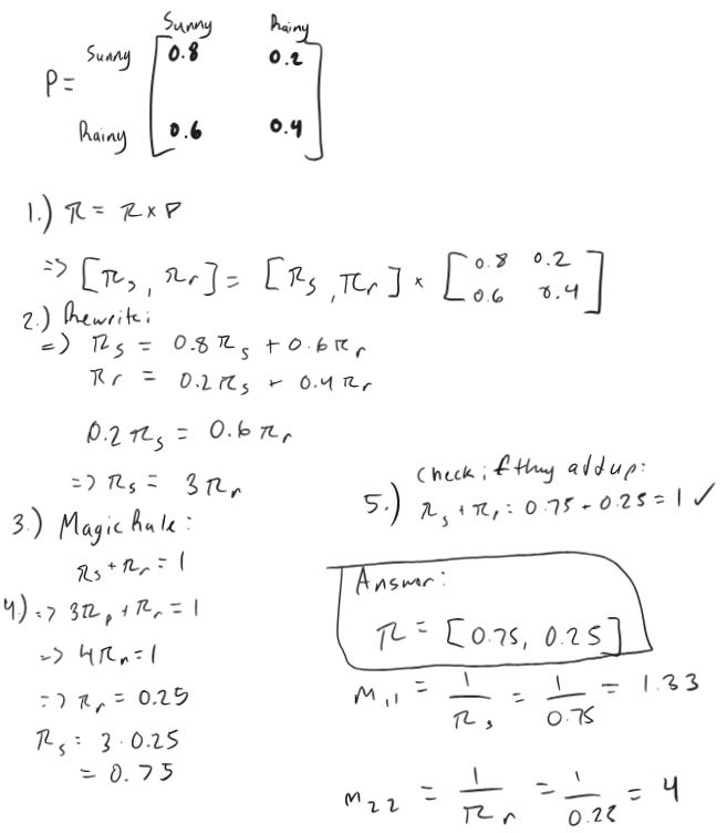
So, since this is probably the most manual part, hopefully these steps help:

1. Write down this equation:

   \(\pi{} = \pi{} \times{P}\)

   1. pi = where you’ll be in the long run

   2. P = transition matrix

2. Rewrite it and just move things around to make it a little easier:

   \(\begin{aligned} \pi{} \times{P} = \pi{} \\ \pi{} \times{P} - \pi{} = 0 \\ \pi{} \times{(P - I)} = 0 \end{aligned}\)

3. Magic rule: when n approaches infinity, where there’s s states:

   \(\pi_1 + \pi_2 + \cdots + \pi_s = 1\)

4. Use algebra to find the values of pi

5. Do all the pi values add up to 1 and are they all between 0 and 1?

Another Example:

Absorbing Chains

---

An absorbing chain is when you have at least one absorbing state inside the chain. Reference the key terms to understand what an absorbing state is. Let’s start off with the Gamblers Ruin:

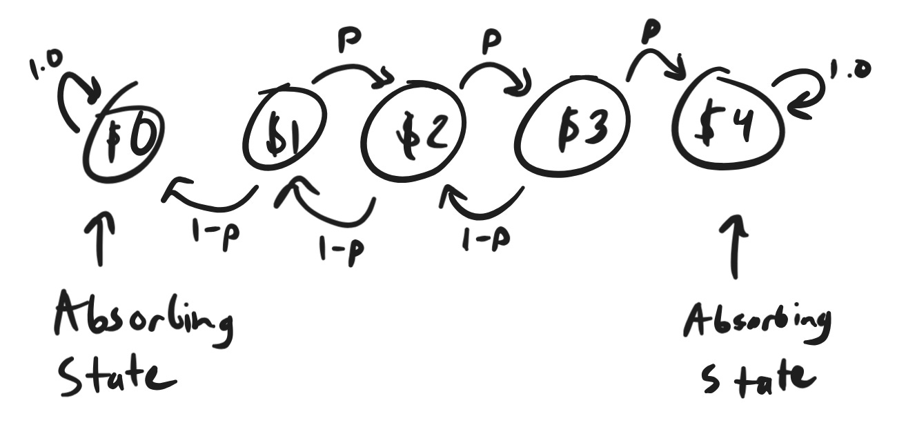
The way Gambler’s Ruin works is that you start out with $1 and you play a game where you either win or lose $1 in each state. Every state represents how much money you have currently and there’s a probability p of winning $1 and probability of 1-p of losing that $1. If you get to $0 or $4, then the game ends there, which is why it’s an absorbing state.

Maybe we want to know what the expected number of times that each state will be entered if the chain begins in a transient state and before we reach an absorbing state, and how many periods we expect to spend in a given transient state before absorption? Maybe we want to know what the probability is that we end up in each absorbing state given that we are in a transient state?

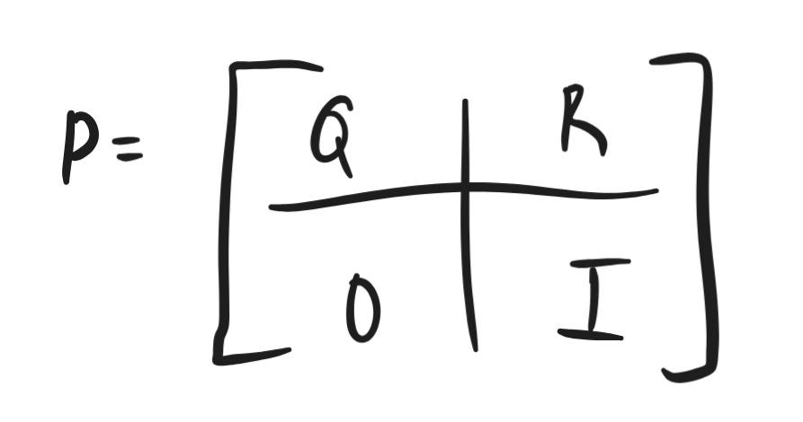
• Q is the transitions between transient states

• R is the transitions from transient states to absorbing states

• 0 is a zero matrix because we can’t leave absorbing states

• I is identity matrix because once we get into an absorbing state, we’re stuck in that state forever.

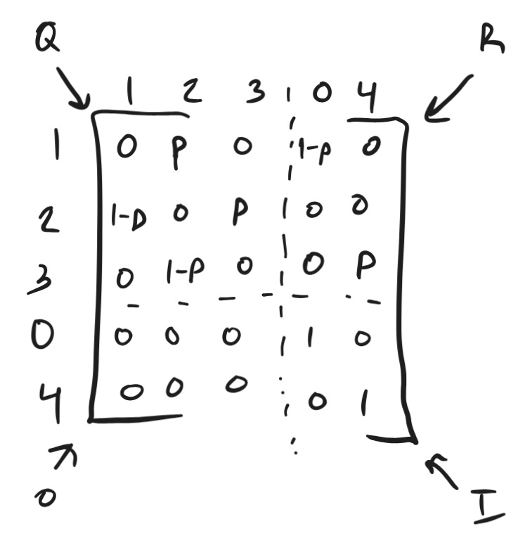
Using the Gambler’s Ruin example, we get this transition matrix. The states in Q are all transient (states 1, 2, and 3) because they can reach $0 and $4 but because states $0 and $4 are absorbing, there is not a path back, so it’s unreachable on the way back to the original state. So, Q just follows are transition diagram on the top of this section, and so does R but we are just using this transition matrix to make things more clearer and to calculate more things later. We have R which is the absorbing states and hopefully we can all see that in the identity matrix I, to get from state 0 to state 0 and from state 4 to state 4 both have a probability of 1 because again they are absorbing states.

To answer our questions, or I guess our curiosity above calculate some things with this matrix, we can use the formula below this to calculate the expected number of periods that will be spent in a transient state before absorption given that we are in another transient state:

\((I-Q)^{-1}\)

This is also called Markov chain’s fundamental matrix.

Note: The I has to have the same dimensions as Q for the calculation to actually work and it’s just an identity matrix, which means just 1’s on the diagonal from top left to bottom right and 0’s everywhere else.

Let’s say p = 0.6, which means 1 - p = 0.4:

\(I - Q = \begin{bmatrix} 1 & -0.6 & 0 \\ -0.4 & 1 & -0.6 \\ 0 & -0.4 & 1 \end{bmatrix}\)

\((I - Q)^{-1} = \begin{bmatrix} 1.46 & 1.15 & 0.69 \\ 0.77 & 1.92 & 1.15 \\ 0.31 & 0.77 & 1.46 \end{bmatrix}\)

This is saying that starting from a certain state that you’ll end up in whatever other state (or the same state) you’re looking at. So, for example, if we start from state one, then we’ll visit state two an average of 1.15 times. If you have $2 now, the expected number of periods that you will be playing is:

\(0.77+1.92+1.15 = 3.84\text{ times}\)

Now, if we want to see what the probability is of ending up at an absorbing state, we use this formula:

\((I-Q)^{-1}\times{R}\)

\((I - Q)^{-1}\times{R} = \begin{bmatrix} 0.58 & 0.42 \\ 0.31 & 0.69 \\ 0.12 & 0.88 \end{bmatrix}\)

So, if we start from state 2, the probability of going broke is 31% and probability of winning $4 is 69%.

If the gambler plays this game 100 times starting with $2 each time, the gambler will lose on average:

\(0.31 \cdot{-$2} + 0.69\cdot{$2} = $0.76 \cdot{100} = $76 \text{profit}\)

If each round of the game takes 5 minutes, how long on average will the gambler play before the game ends, starting with $2? We just find the expected rounds from state two, which is the sum of row two, and multiply it by 5:

\(0.77 + 1.92 + 1.15 = 3.84 \cdot{5} = 19.2 \text{ minutes }\)

If 1,00 gamblers start with $2, then 1,000 x 0.31 = 310 gamblers will go broke.

Starting with $2, the gambler will have exactly $1, 0.77 times on average.

If 100 gamblers start at $2 and play until absorption, the total rounds played would be the sum of the second state row, which is 3.84 rounds per gambler, and multiply that by 100 gamblers = 384 rounds.

If 500 gamblers start at $1 each day, the number of gamblers reaching $4 is 500 gamblers x 0.42 (42% of gamblers) = 210 gamblers.

If the casino pays $50 to the winner at $4, and 200 gamblers start at $3, the casino pays out 0.88 (88% of the gamblers) x 200 gamblers = 176 winners x $50 per winner = $8,800 in total.

That’s about it for Markov Chains for now. The most manual problem would be a steady state problem. This is just an introduction to some Markov Chain topics. We will learn about other Markov Chain topics later.